|
| Mathematics of Backgammon |

Thank you to Douglas Zare and Gammon Village
for their kind permission to reproduce it here.
The problem is that my intuition is all wrong.”
— John Preskill, a professor of physics at Caltech
A Paradox
The doubling cube may escalate so rapidly that the theoretical average value of a position (equity) may not be defined. Backgammon is the only 2-player zero-sum game allowing this possibility. This is a problem for any rigorous theoretical analysis of the whole game of backgammon, since it is unclear whether equity is defined from the initial position. It’s also fun to think about it.
|
| The Paradox Position. |
In this position, whoever rolls a 6 first has a huge advantage. Every entering roll hits a second checker, and probably wins a gammon if not a backgammon. Is the correct cube action from each side redouble/take? If so, the cube may escalate extraordinarily rapidly.
|
| Exact bearoff required. |
Some backgammon variants require you to bear off exactly. Rolling 6-5 would not allow you to bear off here. The first player to roll a 1 wins. Again, the cube may go through the roof.
I would like to highlight some of the strange properties of these positions. Many of the usual analytical tools break down in interesting ways.
Some of the analysis presented here has been done by others. See the rec.games.backgammon archive. I’d like to thank Chris Yep and David Ullrich for their work and helpful discussions.
A Normal Position
|
| Black redoubles. |
This simple position arose in a recent chouette. I faced redoubles to 4 and 16. In theory, the correct decision is to take, since black misses 10/36 of the time. However, I’ve watched people pass in better situations. Perhaps they didn’t know the odds, but perhaps at that instant, the connection between a theoretical number and the right decision seemed tenuous.
I was ahead about 15 points; did I really want to lose 20 points rather than 10 most of the time? Hmmm. If you had to convince a partner who did not trust the math, what could you say?
“We give up more than a point of equity if we pass.”
“I checked at the bar. We can’t buy drinks with equity.”
“If we take this 36 million times, we will win very close to 10 million of those.”
“But we are not going to take this 36 million times. We get this decision in this game only once. And I don’t want to take even this one time.”
“There will be other decisions just like this one. If we use the strategy of taking, we will almost surely end up ahead in the long run.”
“There is no long run. I’m going to use the strategy of not being your partner after this game. If we take now, most of the time we lose today.”
In real life, I had no partner to convince. I trust the math. I took, and the captain kindly rolled 2-1.
I wouldn’t fault you for questioning whether to take if you know the chance of winning is 10/36. After analyzing a situation with a mathematical model, you should ask whether you believe the results. You might find a critical error in the model. Here, for example, you might reject the assumption that the value of money is linear if you realize that you can’t cover a loss, or you recognize that a loss would be more painful for you than a win would be good. You might feel there is extra value in keeping or dodging the box.
In this normal position, every mathematical method works. Everything recommends taking. In positions of undefined equity, different tools may produce different conclusions. It is important not to feel satisfied after finding one answer. It’s good to question the results.
Take or Pass?
We’d like to know the right cube action in the Paradox Position. It’s relatively easy to show that taking must be better than passing.
|
|
Black redoubles. Take or pass? |
White just left a triple shot with a 6-5. If doubled in this position, should white take or pass?
On black’s 9 misses, it’s not obvious whether white should play on for the gammon. White could choose to double, and black would have to pass. After a miss, white is at least as well off as if white exercises this option. So, even if you don’t know whether white should cash or play on, you can conclude that it is right to take. (The real question should be whether black should redouble.)
|
| The Paradox Position |
Similarly, in the Paradox Position, if black redoubles, then white definitely should take.
Taking and never redoubling is better than passing if rolling the first 6 is worth less than 2.7 cubeless. Although a backgammon is a real possibility, closing out 5 checkers usually wins just under 50% backgammons, and a closeout is far from certain. Rolling a 6 is worth less than 2.0 cubeless, so taking and never redoubling is better than passing. Redoubling later might be better, or it might not, but taking is clear.
Redouble?
In the Paradox Position, should the player on roll always redouble? How much is the position worth? These questions are at the heart of the paradox. It is difficult to answer these questions, and many standard methods break down. Let me admit before starting that after all of the analysis, I don’t know how much the Paradox Position should be worth, and I don’t know whether it is right to redouble.
In most positions, you can estimate the average points won by black, and subtract the average points won by white. Here, if both players redouble when possible, the cube escalates so rapidly that both black and white win infinitely many points on average. Subtracting infinity from infinity usually doesn’t give a sensible answer. So, we turn to other techniques.
Strategy versus Strategy
Maybe redoubling is wrong. In a normal game of backgammon from the initial position, it doesn’t seem right to redouble every turn, but if two players decided to redouble whenever legally possible, it might be that the average points won by each side would be infinite, too. That wouldn’t mean the redoubles were correct, or that this would have anything to do with the value of the position if it were played correctly.
How can you refute the idea that doubling at every opportunity is right in normal backgammon? If I found a player who always doubled whenever it was legally possible, my wins would be finite, but large. I would hold the cube until I had an overwhelming advantage, so my wins would be magnified while my losses would tend to be 2 points. I might not win the most possible, and I can’t quantify the player’s average losses, but my strategy would punish the strategy of always doubling. Is there a similar way to punish always redoubling in the Paradox Position?
Suppose we are willing to redouble up to n times, then we chicken out and stop redoubling. Call this the n-brave strategy. Never doubling is the 0-brave strategy, and always doubling is the infinity-brave strategy. We’ll call that the maniac strategy. How do these strategies fare against each other?
For simplicity, we’ll assume that the value of rolling the first 6 is 2, like winning a gammon, regardless of the location of the cube.
|
First Roller | Second Roller | |||||||
| 0 | 1 | 2 | 3 | 4 | 5 | 6 | maniac | |
| 0 | .361 | .361 | .361 | .361 | .361 | .361 | .361 | .361 |
| 1 | .721 | .220 | .220 | .220 | .220 | .220 | .220 | .220 |
| 2 | .721 | .916 | −.050 | −.050 | −.050 | −.050 | −.050 | −.050 |
| 3 | .721 | .916 | 1.292 | −.572 | −.572 | −.572 | −.572 | −.572 |
| 4 | .721 | .916 | 1.292 | 2.017 | −1.579 | −1.579 | −1.579 | −1.579 |
| 5 | .721 | .916 | 1.292 | 2.017 | 3.415 | −3.521 | −3.521 | −3.521 |
| 6 | .721 | .916 | 1.292 | 2.017 | 3.415 | 6.112 | −7.267 | −7.267 |
| maniac | .721 | .916 | 1.292 | 2.017 | 3.415 | 6.112 | 11.315 | ??? |
The player willing to put in the last redouble has an advantage. Indeed, if both sides are willing to redouble at least twice, being willing to make the last redouble is more important than getting to roll first. Against someone willing to redouble to a higher level than you, you do better not to redouble at all, and every redouble you make hurts you.
If you throw out the maniac strategy, no strategy dominates another. That is, for any n and m, there is a strategy against which the n-brave strategy does better, and there is another strategy against which the m-brave strategy does better. As long as a maniac does not encounter another maniac, the maniac does better than the rest. The n-brave strategies don’t refute the maniac strategy; they get destroyed by it!
I think we can’t ignore the maniac strategy, and there is reason to consider it better than the n-brave strategies, but I’m not convinced that the maniac strategy is best.
If a maniac plays against another maniac, the average result is undefined. Perhaps this means the maniacal strategy should be classified as a nonstrategy, just as logicians say that, “This statement is false.” is not a statement. I’m not sure.
I believe the mathematical model of backgammon breaks down. Though always redoubling beats any strategy of redoubling n times and then stopping, you can’t execute the strategy of always redoubling. At some point before there are quadrillions of dollars nominally at stake, you can’t pay if you lose and you won’t get paid if you win. It could be that a better model of backgammon would conclude that the 0-brave or 10-brave strategy is optimal in a more restricted context.
Algebra
|
|
Double match point. Black on roll. |
Black has an outside prime and a desperation shot at white’s 15th checker. Suppose we want to determine the probability with which black hits, p. This is greater than 11/36, since if black misses, white may roll 1-1, and the position would essentially repeat. To approximate p, we can state this in algebra, then solve the equation.
| 11 |
| 36 |
| 25 |
| 36 |
| 1 |
| 36 |
| 396 |
| 1271 |
This gives us the right answer. Can we use the same technique to assign an equity to the Paradox Position, assuming that both sides always redouble?
Let C be the value of rolling the first 6. C is a bit less than 2.
| 11 |
| 36 |
| 25 |
| 36 |
| 11 |
| 43 |
If C ≅ 2, that is about .5. Algebra provides the answer, right?
Algebra provides an answer, but the answer it gives us is meaningless.
Let’s change the situation slightly. I roll first. If I roll the first 6, I get C, but if you roll a 6 first, you get ten percent more, 1.1 C. This is an improvement for you, right? Let’s see what the algebra says.
| 11 |
| 36 |
| 25 |
| 36 |
| 11 |
| 36 |
| 25 |
| 36 |
| 209 |
| 602 |
If C ≅ 2, this is about .7. The algebra says my equity has increased. However, the difference between the two situations is that you get more when you roll the first 6, so my equity should decrease. The algebra is wrong. The number seems ok at first, but it doesn’t mean anything. What is going on?
Some manipulations of symbols on a page don’t make sense, and we’ve encountered one. Suppose you win 4n with probability 1/2n for n = 1, 2, 3, etc.; perhaps I toss a coin until it shows heads, and pay you 4n if the first head is on the nth toss. How much is this worth? The expected value coming from the nth possible win is
| 1 |
| 2n |
So we could write:
This is nonsense. You always win something, so the value can’t be negative. You can say the sum is +∞, but not −2. This type of nonsensical summation of all positive terms is behind the result that improving your payoff from C to 1.1 C decreases your equity. The algebraic method does not evaluate the Paradox Position.
A Capped Cube
Many novices assume that the cube can’t escalate beyond 64, since that is the largest number on the doubling cube. Most of the time, this makes no difference, just as it makes little difference whether someone understands en passant captures in chess.
The paradoxes come from the ability of the cube to escalate without bound, so we could resolve the Paradox Position if we limited the cube to 64 or 1024. What happens if we set a cap on the cube, then let that cap increase? If the prescribed action and value of the position settle down, maybe those should be the answers.
Let’s suppose that gammons and backgammons count even on the maximum cube value, and there is no value to using the cube after someone rolls a 6. For simplicity, let’s assume that rolling the first 6 always wins a gammon, so it is worth twice the value of the cube. Under these assumptions, the equities can be calculated exactly. The following table assumes that the cube starts on 2, but the equities are expressed in EMG.
| Cap | Action | Never Redouble | Redouble/Take |
| 4 | Redouble | .0361 | .721 |
| 8 | No Redouble | .0361 | .220 |
| 16 | Redouble | .0361 | .721 |
| 32 | No Redouble | .0361 | .220 |
| 64 | Redouble | .0361 | .721 |
| 128 | No Redouble | .0361 | .220 |
| 256 | Redouble | .0361 | .721 |
| 512 | No Redouble | .0361 | .220 |
In the Paradox Position, even when the cube is on 2, it matters a lot whether you can redouble to 512 or only to 256. In fact, it appears that you should not redouble if your opponent would be the one to redouble to the highest level. There is a big advantage to being able to make the last redouble.
Suppose the cube can’t go above 16. If your opponent redoubles to 4, you have to take, but the above table suggests that you should never redouble again. Maybe you should beaver! If you beaver to 8, you get to make the last redouble, to 16.
| Cap | Action | Never Redouble | Redouble/Take | Redouble/Beaver |
| 4 | Redouble | .0361 | .721 | — |
| 8 | No Redouble | .0361 | .220 | 1.443 |
| 16 | Redouble | .0361 | .721 | .441 |
| 32 | No Redouble | .0361 | .610 | 1.443 |
| 64 | Redouble | .0361 | .375 | 1.220 |
| 128 | No Redouble | .0361 | .701 | .750 |
| 256 | Redouble | .0361 | .248 | 1.403 |
| 512 | No Redouble | .0361 | .721 | .496 |
Strangely enough, with a capped cube, the correct cube action may be redouble/beaver! Beavers don’t mean that the second player has an advantage. With a capped cube, beavering may allow a player to use the cube in the future, while taking would mean the player could not profitably redouble. Beavering may reduce the advantage of the player on roll. With the cap at 512, the following actions are optimal, assuming each side keeps missing.
| Opponent | You |
| Redouble to 4 | Beaver to 8, Redouble to 16 |
| Take, Redouble to 32 | Take, Redouble to 64 |
| Take, Redouble to 128 | Beaver to 256, Redouble to 512 |
| Take |
The precise actions depend on the value of rolling a 6 first and on the cap. If the value of rolling the first 6 were 3, then it would be right to pass with the cube capped at some levels, and beaver at other levels. If this agrees with your intuition, you may need to see a doctor.
Since the equity and correct cube actions change with the cap, the capped game doesn’t tell us what is right in the Paradox Position without a cap.
The Law of Large Numbers
If you roll a die, the expected value is 3.5. Of course, you would be very surprised if you rolled exactly 3.5 pips, but the average of the possibilities is 3.5. This is true even if you are only allowed to roll the die once. However, one consequence is that if you repeat the roll many times, the probability that the average is between 3.4 and 3.6 is over 90%. If you roll the die enough times, the average will be arbitrarily close to 3.5 with a probability arbitrarily close to 100%. This is called the Law of Large Numbers.
If both players redouble at every opportunity in the Paradox Position, the expected value does not exist because the expected wins for both sides are infinite, and it doesn’t make sense to subtract infinity from infinity. Then again, in second grade I was told that you can’t subtract 4 from 2, but later was told −2 is an acceptable answer. Perhaps there is a number we can associate to the Paradox Position using the idea of the Law of Large Numbers.
Let’s play the Paradox Position many times as a prop and total the results. If the average result gets closer to .3, then we can say the value of the Paradox Position is about .3. However, strange things happen instead.
As a control, let’s consider rolling a die. We could roll the die 10 times. We would expect to get a total of 35, but 1 time in 100, we would get a total of 23 or less. 1 time in 10, we would get a total of 28 or less. The following table shows some of the percentiles of the sums of batches of 10, 100, 1000, and 10,000 dice.
| Percentile (exact) | |||||
| 1st | 10th | 50th | 90th | 99th | |
| 10 | 23 | 28 | 35 | 42 | 47 |
| 100 | 310 | 328 | 350 | 372 | 390 |
| 1,000 | 3,374 | 3,431 | 3,500 | 3,569 | 3,626 |
| 10,000 | 34,603 | 34,781 | 35,000 | 35,219 | 35,397 |
If we use an experimental approach to determining the average value of a die, then by 100 trials, more than 98% of the time our estimate will be between 3 and 4. After 10,000 trials, more than 98% of the time our estimate will be between 3.46 and 3.54. The median result (50th percentile) is close to the expected result of 3.5 per die.
The Petersburg Paradox
To warm up for the Paradox Position, let’s consider the Petersburg Paradox: You win 2 with probability 1⁄2, 4 with probability 1⁄4, etc. The average win is infinite, but you won’t see this in a finite number of trials. If you play the game 10 times, it is possible to win a huge amount, but most of the time you won’t. Half the time, you win 58 or less in 10 trials. There is a small chance of a huge win.
| Percentile (exact or from numerical trials) | |||||
| 1st | 10th | 50th | 90th | 99th | |
| 10 | 24 | 30 | 58 | 190 | 1,364 |
| 100 | 464 | 588 | 920 | 2,528 | 17,174 |
| 1,000 | 7,651 | 9,066 | 12,558 | 27,418 | 146,778 |
| 10,000 | 109,232 | 123,578 | 158,798 | 300,382 | 1,503,126 |
This looks very different from Experiment A. The typical value per trial increases as the number of trials increases! If you play the Petersburg Paradox game 10 times, most of the time you get less than 6 per trial. After 10,000 trials, the median result is about 16 per trial. The results don’t converge. In fact, after n trials, the median and any fixed percentile grow as c n log n, or c log n per trial.
Let’s consider a single batch of 10,000 trials of the Petersburg Paradox. Out of 10,000, how many trials end at each level?
| 4,974 | times, | the payoff was | 2, | for a total of | 9,948. |
| 2,562 | times, | the payoff was | 4, | for a total of | 10,248. |
| 1,276 | times, | the payoff was | 8, | for a total of | 10,208. |
| 591 | times, | the payoff was | 16, | for a total of | 9,456. |
| 305 | times, | the payoff was | 32, | for a total of | 9,760. |
| 151 | times, | the payoff was | 64, | for a total of | 9,664. |
| 61 | times, | the payoff was | 128, | for a total of | 7,808. |
| 38 | times, | the payoff was | 256, | for a total of | 9,728. |
| 17 | times, | the payoff was | 512, | for a total of | 8,704. |
| 9 | times, | the payoff was | 1,024, | for a total of | 9,216. |
| 8 | times, | the payoff was | 2,048, | for a total of | 16,384. |
| 6 | times, | the payoff was | 4,096, | for a total of | 24,576. |
| 1 | time, | the payoff was | 8,192, | for a total of | 8,192. |
| 0 | times, | the payoff was | 16,384, | for a total of | 0. |
| 1 | time, | the payoff was | 32,768, | for a total of | 32,768. |
| 0 | times, | the payoff was | greater, | for a total of | 0. |
The average payoff for each level is the same, 10,000. However, it is atypical for any trial to have a payoff over 216 = 65,536. The probability that a particular trial pays over 65,536 is 1/65,536, so in 10,000 trials, the expected number of payoffs greater than 65,536 is 10,000/65,536. The probability of at least one is only 14%, so over 85% of the time there is no payoff greater than 65,536. Therefore, the possibility of a payoff greater than 65,536 does not affect the median result much.
In a typical batch of 10,000, there are 12 to 15 levels represented (log2 10,000 ≅ 13.3), and the total payoff for each level is roughly 10,000.
In a batch of 1,000,000 trials, it would be unusual not to have several trials paying more than 216. Paying more than 223 would be unusual. More payoff levels typically contribute to the average payoff, so the median result is higher per trial. Experimentally, we would associate a higher value to the Petersburg Paradox game after more trials. Extending a rollout of the Petersburg Paradox doesn’t just decrease the noise, it affects the median result. (For more details, see Martin-Lvf, Anders. “A limit theorem which clarifies the ‘Petersburg paradox’.” Journal of Applied Probability 22 (1985), no. 3, 634643.)
The Paradox Position
|
| The Paradox Position. |
Now, let’s consider the Paradox Position. Again, we’ll consider the total after 10 to 10,000 trials, with the same player redoubling to 4 at the start of each trial.
| Percentile (from numerical trials) | |||||
| 1st | 10th | 50th | 90th | 99th | |
| 10 | −523,832 | −4,040 | +4 | +4,132 | +262,792 |
| 100 | −33,550,028 | −461,588 | −32 | +272,920 | +17,037,304 |
| 1,000 | −2,148,303,152 | −32,755,448 | −2,960 | +19,332,100 | +1,333,668,100 |
| 10,000 | −137,556,832,076 | −2,140,526,756 | −175,796 | +1,445,464,948 | +274,418,671,588 |
The first line of this table shows how dangerous it can be to play out the Paradox Position a few times. Even if you play for $0.01 per point, it isn’t a big surprise to win or lose thousands of dollars in the first 10 trials.
The result of playing the Paradox Position many times is even stranger than the Petersburg Paradox. The median result of the batches of 10,000 was to lose 17.6 points per trial, and the 1st and 99th percentiles involved wins and losses of over 10 million points per trial.
The results after 10,000 trials appear astronomical, but there is a method to the madness. It may not be a huge surprise to win 100 billion points, but it would be a big surprise to win 100 trillion points. If you play 36/25 as much, the typical largest cubes double in size. Since the smaller cubes become negligible, the total results after 36/25 as many trials are about −2 times as great. After n trials, the result is roughly proportional to
After n trials, it is quite unusual for the wins or losses to exceed 10,000 n1.901.
Why is the median result negative after 10,000 trials? It could be that this just statistical noise, but I used 99,999 batches of 10,000. The median of the samples is between the 49.5th and 50.5th percentiles with high confidence. When the number of trials is large, multiplying the number of trials by 36/25 multiplies the median total by about -2. So, even if the median after 10,000 trials were positive, the median after 14,400 trials should be negative.
| n | Median | Sign |
| 50 | −4 | − |
| 60 | 60 | + |
| 70 | 28 | + |
| 80 | 116 | + |
| 100 | −32 | − |
| 120 | 192 | + |
| 140 | 56 | + |
| 160 | 400 | + |
| 200 | −52 | − |
| 240 | 264 | + |
| 280 | −692 | − |
The repetition of the signs −, +, +, + from 50–80 and 100–160 agrees with the idea that the signs oscillate from positive to negative and back as the number of trials increases from n to (36/25)2 n = 2.0736 n. The pattern isn’t followed perfectly, but the data isn’t perfect, either.
This type of reversal happens elsewhere, too. Suppose a strong player plays in a series of backgammon tournaments. After a small number of tournaments, even the strongest players are unlikely to win, so the median result is to lose. After hundreds of tournaments, it would be atypical for a strong player not to win many tournaments, so the median result is to win.
Suppose a strong tournament player has a small chance to steam and lose tens of thousands of points in the side chouettes, far more than is at stake in the tournament itself. If the chance of this disaster is small, it may take thousands of tournaments to arise, but eventually the absence of a disaster would be atypical. It may be that after thousands of tournaments, the median total would become negative again. In the Paradox Position, this repeats indefinitely.
Another possible example of this occurs in backgammon error rates/advantages. It is difficult to determine an error rate because players may play well for a long time, then make extremely large errors in unusual positions. These may contribute significantly to the players’ error rates, particularly against opponents who aim for these types of positions. The median error rate after a few matches may be significantly lower than the typical error rates after hundreds of matches.
Match Play
In match play, it is impossible to have a legal position with an undefined equity. The cube can’t meaningfully escalate to infinitely many levels. In theory, we should be able to determine the correct cube action in match play.
Match play usually resembles money play when the cube is very small compared with the number of points both players need to win. There is no guarantee that this is true in the Paradox Position, since there is a substantial chance that the cube will escalate to the maximum level before someone rolls a 6 if both players double at each opportunity.
If rolling the first 6 is worth a single win, there are only six even match scores at which it is wrong to double within the 15-point match. When both players need 3 or 4 points, it is wrong to double. The redouble at these match scores is much more powerful than the initial double, so doubling offers your opponent a more powerful weapon too frequently. When both players need 7, 8, 9, or 10 points, it is wrong to redouble to 4. The redouble to 8 at these match scores is particularly powerful, and redoubling to 4 makes too many losses worth 8 points. The possibility of redoubling to 16 afterwards is a very weak threat. It appears to be wrong to double from the center from 16-away 16-away to 25-away 25-away, but right to make redoubles at all levels.
In the Paradox Position, the player who rolls a 6 first doesn’t always win, but usually wins a gammon, and sometimes a backgammon. Suppose rolling the first 6 wins a single game 25% of the time, and a gammon 75% of the time. This increases the power of the double to 2 at 3-away 3-away and 4-away 4-away because doubling threatens to win the match with a doubled gammon. The power of the redouble to 4 is weakened at these scores, since the redouble kills gammons. So, it is right to double at these match scores. It is wrong to double to 2 at only two even match scores within a 25-point match, 7-away 7-away and 8-away 8-away. At those scores, the gammonish redoubles to 4 are too powerful. It’s right to redouble to 4 or 8 at any even match score, and wrong to redouble to 4 or 8 with any lead.
I’m not sure whether the Paradox Position has subtleties in longer matches analogous to the oscillations in the correct cube action with a capped cube in Part 1. This may depend on some fundamental questions about the asymptotics of the match equity table. Specifically, at which scores and cube levels does the doubling cube fail to roughly double the amount of equity at stake? How abruptly does the cube lose power? If the doubling cube weakens gradually, I believe redoubling is always right in the Paradox Position with gammons. It may be that the gain from doubling varies, but that the correct action is always redouble/take.
Table Stakes
When backgammon is played for money online, there is a limit to how much each player can win or lose in a game. Any nominal amount won or lost above this limit is ignored. The limit is always symmetric, so you can’t lose more than your opponent can lose.
On GamesGrid, the table limit is usually a high constant number of points for each game of a session, perhaps 20. Most of the time, the cube stays low, and the limit does not affect the correct plays.
On TrueMoneyGames, people often play until one player has won all of the money brought to the table. When one player has only a few points left, this radically changes the correct cube strategies.
|
|
Table limit 6 points. Black to roll or redouble. |
For money play, this would be too good to redouble and a huge pass. Under table stakes rules, with 6 points remaining for each player, this is not good enough to redouble and an easy take. Redoubling to 8 would kill black’s gammons, and white would be happy to risk 2 points to gain 10 without having to worry about gammons.
In the Paradox Position, even a high table limit may be reached frequently if both players redouble at each opportunity. The value of the table limit is important even when the cube is small.
A table limit of 16 points is closely related to a cap on the cube of 16. It may seem that an important difference in the Paradox Position is that the last redouble kills the gammons. However, to my surprise, this difference makes little qualitative difference, so I will concentrate on a modified Paradox Position with no gammons. (The correct redoubles reverse on powers of 2, though.)
With a limit close to twice the value of the cube and no gammons, doubling is very powerful, since there is no effective redouble. To avoid giving your opponent a good redouble when you fail to roll a 6, you should not redouble when the table limit between 86/25 = 3.44 and 3004/625 = 4.8064. Therefore, redoubling is particularly effective when the table limit is between 6.88 and 9.6128, because your opponent will not be able to redouble correctly, etc. So, intervals in which it is not right to redouble alternate with intervals in which redoubling is correct. The following graph shows this alternation.
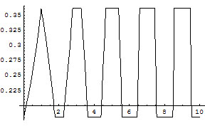
The y-axis is EMG. The x-axis is logarithmic in powers of 2. The troughs surround even powers of 2. It’s not right to redouble when the table limit is close to a power of 4 times the cube level. It is particularly effective to redouble when the table limit is close to 2 times a power of 4. (With gammons, these are reversed.) Everywhere that the graph is above the minimum, the correct action is redouble/take.
A table limit of about 8 times the level of the cube corresponds to the plateau between the 22 and 24. The nonroller can take, and then never use the cube again. A better option, if allowed, is to beaver, even though the roller is still ahead. If a 6 is not rolled, this will let the nonroller redouble. This is a particularly useful tactic when the next redouble will be effective, in the middle of the old plateau. This, and subsequent ramifications, can be seen in the following graph.
Interestingly, it is much rarer for the equity to equal the base of 11/61, which corresponds to keeping the cube. Redoubling is right more frequently. As the graph indicates, the correct strategy is complicated, and is sensitive to proportionately small changes in the table limit.
Not only is there a dip in the middle of the old plateau around 8, but this dip propagates to higher limits. Because of the ability to gain from beavering later, it is right to redouble when the table limit is about 16 times the cube. It is no longer particularly effective to redouble then the table limit is 32 times the cube, and it is actually wrong to double when the limit is 128 times the cube. The potential value of the beaver on a much higher cube completely reverses the effectiveness of the cube when the table limit is 128 times the cube.
Where a peak is followed a factor of 4 later by a dip, the correct action was to beaver. For example, there are two peaks at the edges of the old plateau around 23. These are followed by dips on either side of 25. It’s right to beaver a redouble when the table limit is 26–29 times the initial value of the cube.
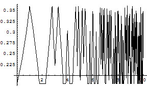
If raccoons were allowed, no beaver would be profitable. This can be seen from the graph with no beavers allowed. Redouble/beaver/raccoon is always better for the roller than redouble/take.
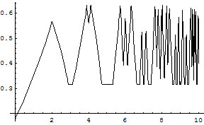
For completeness, here is a graph of the equity when rolling a 6 wins 25% single games and 75% gammons.
Summary
If you play n games of the Paradox Position, with each player doubling, typical results are proportional to n1.901. It is unusual to win or lose more than 10,000 n1.901 points.
Whether the median result is to win or to lose depends on the number of trials. For large n, the sign of the median result oscillates from positive to negative and back as the number of trials increases from n to 2.0736 n.
In match play, it appears to be wrong to double the Paradox Position at 7-away 7-away and 8-away 8-away, but right to double and redouble at all other even match scores within a 25-point match.
With table stakes, the correct cube action may be no redouble/take, redouble/take, or redouble/beaver. If beavers are allowed, it is rarely wrong to redouble, and it is important to beaver at the right times. The strategy is complicated.
After all of these attempts to understand the Paradox Position, I’m not convinced that it is more right to redouble than not to redouble.